Starting With Data
Overview
Teaching: 60 min
Exercises: 30 minQuestions
How can I import data in Python?
What is Pandas?
Why should I use Pandas to work with data?
Objectives
Navigate the workshop directory and download a dataset.
Explain what a library is and what libraries are used for.
Describe what the Python Data Analysis Library (Pandas) is.
Load the Python Data Analysis Library (Pandas).
Use
read_csvto read tabular data into Python.Describe what a DataFrame is in Python.
Access and summarize data stored in a DataFrame.
Define indexing as it relates to data structures.
Perform basic mathematical operations and summary statistics on data in a Pandas DataFrame.
Create simple plots.
Working With Pandas DataFrames in Python
We can automate the process of performing data manipulations in Python. It’s efficient to spend time building the code to perform these tasks because once it’s built, we can use it over and over on different datasets that use a similar format. This makes our methods easily reproducible. We can also easily share our code with colleagues and they can replicate the same analysis.
Starting in the same spot
To help the lesson run smoothly, let’s ensure everyone is in the same directory. This should help us avoid path and file name issues. After launching Spyder (remember you can launch Spyder from the Anaconda Navigator), open the project you created in the previous session. You can do this under the Projects tab.
If you are working in IPython Notebook be sure that you start your notebook in the workshop directory.
A quick aside that there are Python libraries like OS Library that can work with our directory structure, however, that is not our focus today.
Our Data
For this lesson, we will be using rainfall data from eThekwini from December 2017. The files can be downloaded here.
This episode will use the rainfall_combined.csv file. After downloading the file move it to your ‘project/data’ folder. Remember, this is the folder that should keep the raw data.
We are studying the rainfall recorded for rain gauges in the different wards of eThekwini. The dataset is stored as a .csv file: each row holds information for a 5 minute period, and the columns represent:
ID,UT,year, month, day, time, raingauges_id,name, ward_id,region, data
| Column | Description |
|---|---|
| ID | Unique id for the observation |
| UT | unix time of observation |
| year | year of observation |
| month | month of observation |
| day | day of observation |
| time | time of observation |
| raingauges_id | unique id for raingauge |
| name | name of raingauge |
| ward_id | unique id for ward |
| region | name of region |
| data | rainfall in mm |
We can open the rainfall_combined.csv file in a text editor.
The first few rows of our file look like this:
ID,UT,year,month,day,time,raingauges_id,name,ward_id,region,data
1,1512227100,2017,12,2,15:05:00,1,BLUFF RES NO.3,66,Central,0.6
2,1512227400,2017,12,2,15:10:00,1,BLUFF RES NO.3,66,Central,0.8
3,1512227700,2017,12,2,15:15:00,1,BLUFF RES NO.3,66,Central,0.2
4,1512228000,2017,12,2,15:20:00,1,BLUFF RES NO.3,66,Central,0.2
5,1512252000,2017,12,2,22:00:00,1,BLUFF RES NO.3,66,Central,0.0
Pandas in Python
One of the best options for working with tabular data in Python is to use the Python Data Analysis Library (a.k.a. Pandas). The Pandas library provides data structures, produces high quality plots with matplotlib and integrates nicely with other libraries that use NumPy (which is another Python library) arrays.
Remember we can load a library with the import statement and give it a nickname. For example we can import the pandas library using the common nickname pd:
import pandas as pd
To call a function from the pandas library we use pd.FunctionName.
Reading CSV Data Using Pandas
We will begin by locating and reading our rainfall data which are in CSV format.
We can use Pandas’ read_csv function to pull the file directly into a
DataFrame.
So What’s a DataFrame?
A DataFrame is a 2-dimensional data structure that can store data of different
types (including characters, integers, floating point values, factors and more)
in columns. It is similar to a spreadsheet or an SQL table or the data.frame in
R. It has columns, with column headers and rows representing observations. A column needs to be of the same data type, i.e. either numeric or character, but different columns can differ in their data type. That means, pandas DataFrames are ideal to hold observational data tables imported into python.
A DataFrame always has an index (0-based). An index refers to the position of
an element in the data structure.
# note that pd.read_csv is used because we imported pandas as pd
# the 'data/' stands for the subfolder data in our working directory
pd.read_csv("data/rainfall_combined.csv")
The above command yields the output below:
         ID          UT  year  month  day      time  raingauges_id  \
0         1  1512227100  2017     12    2  15:05:00              1
1         2  1512227400  2017     12    2  15:10:00              1
2         3  1512227700  2017     12    2  15:15:00              1
3         4  1512228000  2017     12    2  15:20:00              1
4         5  1512252000  2017     12    2  22:00:00              1
5         6  1512325800  2017     12    3  18:30:00              1
6         7  1512326100  2017     12    3  18:35:00              1
7         8  1512326400  2017     12    3  18:40:00              1
8         9  1512326700  2017     12    3  18:45:00              1
9        10  1512327000  2017     12    3  18:50:00              1
10       11  1512338400  2017     12    3  22:00:00              1
11      334  1512394500  2017     12    4  13:35:00              1
12      349  1512397500  2017     12    4  14:25:00              1
13      350  1512398400  2017     12    4  14:40:00              1
14      485  1512404700  2017     12    4  16:25:00              1
15      486  1512406500  2017     12    4  16:55:00              1
16      487  1512406800  2017     12    4  17:00:00              1
17      670  1512408300  2017     12    4  17:25:00              1
18      671  1512408900  2017     12    4  17:35:00              1
19      672  1512409500  2017     12    4  17:45:00              1
20      673  1512409800  2017     12    4  17:50:00              1
21      674  1512411000  2017     12    4  18:10:00              1
22      990  1512412200  2017     12    4  18:30:00              1
23      991  1512414600  2017     12    4  19:10:00              1
24      992  1512414900  2017     12    4  19:15:00              1
25     1440  1512415200  2017     12    4  19:20:00              1
26     1441  1512415500  2017     12    4  19:25:00              1
27     1442  1512416100  2017     12    4  19:35:00              1
28     1443  1512417000  2017     12    4  19:50:00              1
29     2033  1512421200  2017     12    4  21:00:00              1
    ...         ...   ...    ...  ...       ...            ...
6714  31895  1512554700  2017     12    6  10:05:00             42
6715  31896  1512555000  2017     12    6  10:10:00             42
6716  34545  1512555900  2017     12    6  10:25:00             42
6717  37320  1512562500  2017     12    6  12:15:00             42
6718  37321  1512562800  2017     12    6  12:20:00             42
6719  40201  1512563100  2017     12    6  12:25:00             42
6720  40202  1512563400  2017     12    6  12:30:00             42
6721  40203  1512563700  2017     12    6  12:35:00             42
6722  40204  1512564000  2017     12    6  12:40:00             42
6723  40205  1512564600  2017     12    6  12:50:00             42
6724  49621  1512573900  2017     12    6  15:25:00             42
6725  49622  1512574200  2017     12    6  15:30:00             42
6726  49623  1512574500  2017     12    6  15:35:00             42
6727  49624  1512574800  2017     12    6  15:40:00             42
6728  49625  1512575700  2017     12    6  15:55:00             42
6729  49626  1512576000  2017     12    6  16:00:00             42
6730  49627  1512576300  2017     12    6  16:05:00             42
6731  49628  1512576600  2017     12    6  16:10:00             42
6732  49629  1512576900  2017     12    6  16:15:00             42
6733  49630  1512577200  2017     12    6  16:20:00             42
6734  53117  1512577500  2017     12    6  16:25:00             42
6735  53118  1512577800  2017     12    6  16:30:00             42
6736  53119  1512578100  2017     12    6  16:35:00             42
6737  53120  1512578400  2017     12    6  16:40:00             42
6738  53121  1512578700  2017     12    6  16:45:00             42
6739  53122  1512579000  2017     12    6  16:50:00             42
6740  53123  1512579300  2017     12    6  16:55:00             42
6741  71149  1512597600  2017     12    6  22:00:00             42
6742  71438  1512609300  2017     12    7  01:15:00             42
6743  71621  1512624300  2017     12    7  05:25:00             42

                name  ward_id    region  data
0     BLUFF RES NO.3       66   Central   0.6
1     BLUFF RES NO.3       66   Central   0.8
2     BLUFF RES NO.3       66   Central   0.2
3     BLUFF RES NO.3       66   Central   0.2
4     BLUFF RES NO.3       66   Central   0.0
5     BLUFF RES NO.3       66   Central   0.2
6     BLUFF RES NO.3       66   Central   0.2
7     BLUFF RES NO.3       66   Central   0.4
8     BLUFF RES NO.3       66   Central   0.8
9     BLUFF RES NO.3       66   Central   0.4
10    BLUFF RES NO.3       66   Central   0.0
11    BLUFF RES NO.3       66   Central   0.8
12    BLUFF RES NO.3       66   Central   0.2
13    BLUFF RES NO.3       66   Central   0.2
14    BLUFF RES NO.3       66   Central   0.4
15    BLUFF RES NO.3       66   Central   0.2
16    BLUFF RES NO.3       66   Central   0.2
17    BLUFF RES NO.3       66   Central   0.4
18    BLUFF RES NO.3       66   Central   0.2
19    BLUFF RES NO.3       66   Central   0.2
20    BLUFF RES NO.3       66   Central   0.4
21    BLUFF RES NO.3       66   Central   0.2
22    BLUFF RES NO.3       66   Central   0.2
23    BLUFF RES NO.3       66   Central   0.8
24    BLUFF RES NO.3       66   Central   1.0
25    BLUFF RES NO.3       66   Central   0.2
26    BLUFF RES NO.3       66   Central   0.2
27    BLUFF RES NO.3       66   Central   0.2
28    BLUFF RES NO.3       66   Central   0.2
29    BLUFF RES NO.3       66   Central   0.2
             ...      ...       ...   ...
6714     AMANZIMTOTI       97  Southern   0.4
6715     AMANZIMTOTI       97  Southern   0.2
6716     AMANZIMTOTI       97  Southern   0.2
6717     AMANZIMTOTI       97  Southern   0.4
6718     AMANZIMTOTI       97  Southern   2.0
6719     AMANZIMTOTI       97  Southern   0.4
6720     AMANZIMTOTI       97  Southern   0.2
6721     AMANZIMTOTI       97  Southern   0.2
6722     AMANZIMTOTI       97  Southern   0.2
6723     AMANZIMTOTI       97  Southern   0.2
6724     AMANZIMTOTI       97  Southern   0.2
6725     AMANZIMTOTI       97  Southern   0.2
6726     AMANZIMTOTI       97  Southern   0.2
6727     AMANZIMTOTI       97  Southern   0.2
6728     AMANZIMTOTI       97  Southern   0.2
6729     AMANZIMTOTI       97  Southern   0.4
6730     AMANZIMTOTI       97  Southern   0.4
6731     AMANZIMTOTI       97  Southern   0.2
6732     AMANZIMTOTI       97  Southern   0.6
6733     AMANZIMTOTI       97  Southern   1.4
6734     AMANZIMTOTI       97  Southern   1.6
6735     AMANZIMTOTI       97  Southern   0.6
6736     AMANZIMTOTI       97  Southern   0.4
6737     AMANZIMTOTI       97  Southern   0.6
6738     AMANZIMTOTI       97  Southern   0.4
6739     AMANZIMTOTI       97  Southern   0.4
6740     AMANZIMTOTI       97  Southern   0.2
6741     AMANZIMTOTI       97  Southern   0.0
6742     AMANZIMTOTI       97  Southern   0.2
6743     AMANZIMTOTI       97  Southern   0.2

[6744 rows x 11 columns]
We can see that there were 6749 rows parsed. Each row has 11 columns. The first column is the index of the DataFrame. The index is used to
identify the position of the data, but it is not an actual column of the DataFrame.
It looks like the read_csv function in Pandas read our file properly. However,
we haven’t saved any data to memory so we can work with it. We need to assign the
DataFrame to a variable. Remember that a variable is a name for a value, such as x,
or data. We can create a new object with a variable name by assigning a value to it using =.
Let’s call the imported rainfall data rainfall_df:
rainfall_df = pd.read_csv("data/rainfall_combined.csv")
Notice when you assign the imported DataFrame to a variable, Python does not
produce any output on the screen. We can view the value of the rainfall_df
object by typing its name into the Python command prompt
rainfall_df
which prints contents like above. (We can also look at it in the Variable Explorer tab in top right window.)
Exploring Our rainfall data
Again, we can use the type function to see what kind of thing rainfall_df is:
type(rainfall_df)
<class pandas.core.frame.DataFrame>
As expected, it’s a DataFrame (or, to use the full name that Python uses to refer
to it internally, a pandas.core.frame.DataFrame).
What kind of things does rainfall_df contain? DataFrames have an attribute
called dtypes that answers this:
In [82]: rainfall_df.dtypes
Out[82]:
ID                 int64
UT                 int64
year               int64
month              int64
day                int64
time              object
raingauges_id      int64
name              object
ward_id            int64
region            object
data             float64
dtype: object
All the values in a column have the same type. For example, UT has type
int64, which is a kind of integer. Cells in the UT column cannot have
fractional values, but the data column can, because it has type float64. The object type doesn’t have a very helpful name, but in
this case it represents strings (such as the time, ward name and region).
Useful Ways to View DataFrame objects in Python
There are many ways to summarize and access the data stored in DataFrames, using attributes and methods provided by the DataFrame object.
To access an attribute, use the DataFrame object name followed by the attribute
name df_object.attribute. Using the DataFrame rainfall_df and attribute
columns, an index of all the column names in the DataFrame can be accessed
with rainfall_df.columns.
Methods are called in a similar fashion using the syntax df_object.method().
As an example, rainfall_df.head() gets the first few rows in the DataFrame
rainfall_df using the head() method. With a method, we can supply extra information in the parentheses to control behaviour.
Let’s look at the data using these.
Challenge - DataFrames
Using our DataFrame
rainfall_df, try out the following attributes and methods to see what they return:.columns,.axes,.ndim,.size,.shape,.head(),.tail(),.describe()(Remember you can use
?, e.g.?rainfall_df.head(), to get some information about an attribute in the console or check the pandas documentation)Can you answer the following questions:
How many rows and how many columns are in
rainfall_df?What is the value of
data(i.e. the rainfall) in row 11 and what in the second last row?What is the mean value and what the median of
data?Take note of the output of
.shape- what format does it return the shape of the DataFrame in? (HINT: More on tuples, here)
Calculating Statistics From Data In A Pandas DataFrame
We’ve read our data into Python. Next, let’s perform some quick summary statistics to learn more about the data that we’re working with. We might want to know how many rain periods were recorded in each rain gauge, or how much rainfall was recorded per month. We can perform summary stats quickly using groups. But first we need to figure out what we want to group by.
Let’s begin by exploring our data:
# Look at the column names
rainfall_df.columns
which returns:
Index(['ID', 'UT', 'year', 'month', 'day', 'time', 'raingauges_id', 'name',
       'ward_id', 'region', 'data'],
      dtype='object')
We can access individual columns of rainfall_df by giving the column name in [], e.g. rainfall_df['year'] only shows the content of column year.
Let’s get a list of all the rain gauges in our dataset. The pd.unique function tells us all of the unique values in the name column.
pd.unique(rainfall_df['name'])
which returns:
array(['BLUFF RES NO.3', 'CHATSWORTH RES NO.1', 'CHATSWORTH RES NO.4',
       "CITY ENGINEER'S DEPT", 'CRABTREE S-P-S', 'DUNKELD RES',
       'FIRWOOD RES', 'ISLAND VIEW S-P-S', 'KENNEDY ROAD S-P-S',
       'RIDGE END RES', 'RIDGE VIEW RES', 'SAND PUMP HOPPER',
       'SHERWOOD RES NO.3', 'ST THOMAS RES', 'WENTWORTH RES',
       'WOODLAND RES NO.2', 'DBN NORTH HL RES', 'NEWLANDS RES NO.3',
       'PHOENIX RES NO.1', 'PHOENIX RES NO.4', 'BALLITO', 'HAZELMERE DAM',
       'UMHWWTW', 'CRAWFORD', 'UMH NTH', 'BUFFELS', 'CATO RIDGE',
       'ALVERSTN', 'INANDA DAM', 'WATERFALL', 'HILLCREST', 'SHONGWENI DAM',
       'PINETOWN', 'NAGLE DAM', 'RIVERLEA', 'KLOOF', 'UMLAZI',
       'UMBUMBULU RES', 'ISIPINGO RES', 'UMKDEPOT', 'AMANZIMTOTI',
       'not there'], dtype=object)
Challenge - Statistics
Create a list of unique ward ID’s found in the rainfall data. Call it
ward_names. How many unique wards are there in the data?What is the difference between
len(ward_names)andrainfall_df['ward_id'].nunique()?
Groups in Pandas
We often want to calculate summary statistics grouped by subsets or attributes within fields of our data. For example, we might want to calculate the average rainfall of all rain gauges per ward.
We can calculate basic statistics for all records in a single column using the syntax below:
rainfall_df['data'].describe()
gives output
count    6744.000000
mean        0.372301
std         0.727326
min         0.000000
25%         0.200000
50%         0.200000
75%         0.400000
max        50.000000
Name: data, dtype: float64
We can also extract one specific metric if we wish:
rainfall_df['data'].min()
rainfall_df['data'].max()
rainfall_df['data'].mean()
rainfall_df['data'].std()
rainfall_df['data'].count()
But if we want to summarize by one or more variables, for example ward, we can
use Pandas’ .groupby method. Once we’ve created a groupby DataFrame, we
can quickly calculate summary statistics by a group of our choice.
# Group data by ward
grouped_data = rainfall_df.groupby('ward_id')
The pandas function describe will return descriptive stats including: mean,
median, max, min, std and count for a particular column in the data. Pandas’
describe function will only return summary values for columns containing
numeric data.
# summary statistics for all numeric columns by ward
grouped_data.describe()
# provide the mean for each numeric column by ward
grouped_data.mean()
grouped_data.mean() OUTPUT:
                   ID            UT    year  month       day  raingauges_id  \
ward_id
1        18020.638889  1.512478e+09  2017.0   12.0  4.907407      25.231481
3        18319.781065  1.512494e+09  2017.0   12.0  5.195266      33.585799
7        18090.628205  1.512497e+09  2017.0   12.0  5.160256      29.000000
8        17605.616766  1.512504e+09  2017.0   12.0  5.287425      28.000000
9        18513.102310  1.512508e+09  2017.0   12.0  5.257426      26.498350
10       16877.924812  1.512502e+09  2017.0   12.0  5.236842      41.000000
11       16036.218182  1.512503e+09  2017.0   12.0  5.272727      11.000000
18       17239.863014  1.512504e+09  2017.0   12.0  5.287671      30.000000
23       18957.900000  1.512517e+09  2017.0   12.0  5.435294       7.000000
24       15715.173913  1.512500e+09  2017.0   12.0  5.233696      14.000000
25       17748.812500  1.512511e+09  2017.0   12.0  5.369318      10.000000
26       20919.337884  1.512512e+09  2017.0   12.0  5.433447       8.242321
27       18760.876289  1.512510e+09  2017.0   12.0  5.386598      13.000000
30       18377.897321  1.512511e+09  2017.0   12.0  5.366071      16.000000
31       19275.084577  1.512510e+09  2017.0   12.0  5.378109      17.000000
32       18716.340000  1.512509e+09  2017.0   12.0  5.365000       5.000000
35       19946.142119  1.512507e+09  2017.0   12.0  5.333333      32.757106
36       16955.581395  1.512504e+09  2017.0   12.0  5.319767       6.000000
52       18899.636364  1.512511e+09  2017.0   12.0  5.351515      20.000000
59       18788.023810  1.512510e+09  2017.0   12.0  5.321429      44.000000
60       17476.962963  1.512506e+09  2017.0   12.0  5.248677      22.000000
63       15829.840580  1.512500e+09  2017.0   12.0  5.246377       8.000000
64       16842.975000  1.512501e+09  2017.0   12.0  5.265000      19.000000
66       17845.055195  1.512498e+09  2017.0   12.0  5.256494       5.077922
68       17649.830189  1.512497e+09  2017.0   12.0  5.213836      18.000000
70       16990.219048  1.512505e+09  2017.0   12.0  5.314286       2.000000
71       16544.668639  1.512506e+09  2017.0   12.0  5.284024       3.000000
80       17146.422886  1.512502e+09  2017.0   12.0  5.273632      32.000000
93       19813.664557  1.512499e+09  2017.0   12.0  5.246835      34.000000
97       17301.702970  1.512497e+09  2017.0   12.0  5.188119      42.000000
99       15659.019355  1.512501e+09  2017.0   12.0  5.187097      35.000000
103      18707.295181  1.512506e+09  2017.0   12.0  5.289157      25.000000
110      16830.762195  1.512505e+09  2017.0   12.0  5.323171      12.000000

             data
ward_id
1        0.229630
3        0.262722
7        0.342308
8        0.241916
9        0.329373
10       0.384211
11       0.385455
18       0.417352
23       0.394118
24       0.333696
25       0.646591
26       0.359044
27       0.370103
30       0.404464
31       0.382090
32       0.389000
35       0.441344
36       0.381395
52       0.533333
59       0.395238
60       0.483598
63       0.440580
64       0.330000
66       0.360390
68       0.290566
70       0.340000
71       0.282840
80       0.366169
93       0.321519
97       0.364356
99       0.317419
103      0.302410
110      0.419512
The groupby command is powerful in that it allows us to quickly generate
summary stats.
Challenge - Summary Data
- How many recorded observations are there in the four different regions?
- What happens when you group by two columns using the following syntax and then grab mean values:
grouped_data2 = rainfall_df.groupby(['day','region'])grouped_data2.mean()- Summarize rainfall values for each day in your data. HINT: you can use the following syntax to only create summary statistics for one column in your data
by_day['data'].describe()Did you get #3 right?
The Output from challenge 3 looks like:
count mean std min 25% 50% 75% max day 1 1.0 0.200000 NaN 0.2 0.2 0.2 0.2 0.2 2 101.0 0.766337 4.969432 0.0 0.0 0.2 0.2 50.0 3 186.0 0.350538 0.576030 0.0 0.2 0.2 0.4 4.8 4 832.0 0.227163 0.130103 0.0 0.2 0.2 0.2 1.2 5 2250.0 0.419200 0.516775 0.0 0.2 0.2 0.4 7.2 6 3308.0 0.368017 0.338559 0.0 0.2 0.2 0.4 5.0 7 66.0 0.278788 0.232389 0.2 0.2 0.2 0.2 1.8
Quickly Creating Summary Counts in Pandas
Let’s next count the number of samples for each raingauge. We can do this in a few
ways, but we’ll use groupby combined with the count() method.
# count the number of samples by raingauge
raingauge_counts = rainfall_df.groupby('raingauges_id')['ID'].count()
print(raingauge_counts)
Did you notice how we combined all the methods into one statement?
Or, we can also count just the rows that have the raingauge “5”:
rainfall_df.groupby('raingauges_id')['ID'].count()[5]
Challenge - Make a list
What’s another way to create a list of raingauges and associated
countof the records in the data? Hint: you can performcount,min, etc functions on groupby DataFrames in the same way you can perform them on regular DataFrames.
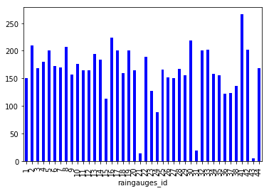
Quick and Easy Plotting Data Using Pandas
We can plot our summary stats using Pandas, too.
Let’s plot our counts per raingauge we just calculated:
# Make sure figures appear inline in Ipython Notebook
%matplotlib inline
# Create a quick bar chart
raingauge_counts.plot(kind='bar')
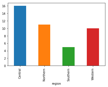
We can also look at how many raingauges are there in each region:
raingauges_region = rainfall_df.groupby('region')['raingauges_id'].nunique()
# Let's plot that too
raingauges_region.plot(kind='bar')
Challenge - Plots
Create a plot with the average or the sum (or both) of rainfall per day over all raingauges.
Mutating columns
If we wanted to, we could perform math on an entire column of our data. For example let’s multiply all rainfall values by 2 or take the log of rainfall. Remember if we want to apply a function to all elements in an array like object we can use functions from numpy, e.g. np.log().
# multiply all rainfall values by 2
rainfall_df['data']*2
# take the log of all values
np.log(rainfall_df['data'])
We can create a new variable for the ‘mutated’ rainfall or adding it as a new column to our dataframe rainfall_df:
# adding the column `ln_data` to `rainfall_df`
rainfall_df['ln_data'] = np.log(rainfall_df['data'])
rainfall_df.head()
A more practical use of this might be to normalize the data according to a mean, area, or some other value calculated from our data.
A few words on dates
Dates in python are represented by date, time and datetime objects from the ‘datetime’ module.
import datetime as dt
# a date
dt.date(year = 2018, month = 1, day = 11)
# a time
dt.time(hour = 9, minute=30, second=15)
# a datetime
dt.datetime(2018, 1, 11, 9, 30, 15)
A defined format for date is important when calculating e.g. differences between dates etc.
Let’s try:
dt1 = dt.datetime(2018, 1, 11, 9, 30, 0)
dt2 = dt.datetime(2018, 1, 11, 10, 0, 0)
dt2 - dt1
datetime.timedelta(0, 1800)
This yields a timedelta object with a value of 1800. datetime objects are represented in seconds, so the difference is given in seconds, and 1800 sec = 30 min.
Now back to our rainfall data. The date and time is represented by the unix time (UT) on the one hand and the columns year, month, day, and time on the other hand. To create a datetime column, Pandas has the function to_datetime:
We can combine year, month and day to a date.
pd.to_datetime(rainfall_df[['year', 'month', 'day']])
We can also convert the unix time into a datetime object:
rainfall_df['datetime']=pd.to_datetime(rainfall_df['UT'], origin='unix', unit='s')
rainfall_df.dtypes
...
datetime         datetime64[ns]
...
Challenge - datetime objects
Add a column with hours to rainfall_df.
HINT: look into the documentation of methods for Pandas Series on how to access individual date and time elements from the
datetimecolumn.
Key Points
pd.read_csv() is used to import tabular data into python
methods to inspect dataframes are .dtypes, .shape(), .head(), .tail()
individual columns from a dataframe can be chosen using [‘ColumnName’]
methods for basic statistics on dataframes are .describe(), .min(), .max(), .mean(), …
.groupby() can be used to group a dataframe by categories
the datetime package offers functionality for datetime objects