Indexing, Slicing and Subsetting DataFrames in Python

Overview

Teaching: 30 min
Exercises: 30 min

Questions

How can I access specific data within my data set?

How can Python and Pandas help me to analyse my data?

Objectives

Describe what 0-based indexing is.

Manipulate and extract data using column headings and index locations.

Employ slicing to select sets of data from a DataFrame.

Employ label and integer-based indexing to select ranges of data in a dataframe.

Reassign values within subsets of a DataFrame.

Create a copy of a DataFrame.

Query /select a subset of data using a set of criteria using the following operators: =, !=, >, <, >=, <=.

Locate subsets of data using masks.

Describe BOOLEAN objects in Python and manipulate data using BOOLEANs.

In lesson 01, we read a CSV into a Python pandas DataFrame. We learned:

how to save the DataFrame to a named object,
how to perform basic math on the data, and
how to calculate summary statistics

In this lesson, we will explore ways to access different parts of the data using:

indexing,
slicing, and
subsetting.

Loading our data

We will continue to use the rainfall dataset that we worked with in the last lesson. Let’s reopen and read in the data again:

# Make sure pandas is loaded
import pandas as pd

# read in the rainfall csv
rainfall_df = pd.read_csv("data/rainfall_combined.csv")

Indexing and Slicing in Python

We often want to work with subsets of a DataFrame object. There are different ways to accomplish this including: using labels (column headings), numeric ranges, or specific x,y index locations.

Selecting data using Labels (Column Headings)

We use square brackets [] to select a subset of an Python object. For example, we can select all data from a column named raingauges_id from the rainfall_df DataFrame by name. There are two ways to do this:

# TIP: use the .head() method we saw earlier to make output shorter
# Method 1: select a 'subset' of the data using the column name
rainfall_df['raingauges_id']

# Method 2: use the column name as an 'attribute'; gives the same output
rainfall_df.raingauges_id

We can also create a new object that contains only the data within the raingauges_id column as follows:

# creates an object, rainfall_raingauges, that only contains the `raingauges_id` column
rainfall_raingauges = rainfall_df['raingauges_id']

We can pass a list of column names too, as an index to select columns in that order. This is useful when we need to reorganize our data.

NOTE: If a column name is not contained in the DataFrame, an exception (error) will be raised.

# select the raingauges and ward columns from the DataFrame
rainfall_df[['raingauges_id', 'ward_id']]

# what happens when you flip the order?
rainfall_df[['ward_id', 'raingauges_id']]

#what happens if you ask for a column that doesn't exist?
rainfall_df['wards']

Python tells us what type of error it is in the traceback, at the bottom it says KeyError: 'wards' which means that wards is not a column name (or Key in the related python data type dictionary).

Extracting Range based Subsets: Slicing

REMINDER: Python Uses 0-based Indexing

Let’s remind ourselves that Python uses 0-based indexing. This means that the first element in an object is located at position

This is different from other tools like R and Matlab that index elements within objects starting at 1.

# Create a list of numbers:
a = [1, 2, 3, 4, 5]

indexing diagram slicing diagram

Challenge - Extracting data
What value does the code below return?
a[0]
How about this:
a[5]
In the example above, calling a[5] returns an error. Why is that?
What about?
a[len(a)]

Slicing Subsets of Rows in Python

Slicing using the [] operator selects a set of rows and/or columns from a DataFrame. To slice out a set of rows, you use the following syntax: data[start:stop]. When slicing in pandas the start bound is included in the output. The stop bound is one step BEYOND the row you want to select. So if you want to select rows 0, 1 and 2 your code would look like this:

# select rows 0, 1, 2 (row 3 is not selected)
rainfall_df[0:3]

The stop bound in Python is different from what you might be used to in languages like Matlab and R.

# select the first 5 rows (rows 0, 1, 2, 3, 4)
rainfall_df[:5]

# select the last element in the list
# (the slice starts at the last element,
# and ends at the end of the list)
rainfall_df[-1:]

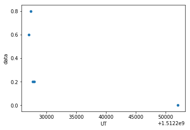
Select the first 5 rows and plot rainfall over UT as points:

rainfall_df[0:5].plot(x='UT',y='data',kind = 'scatter')

scatter plot

We can also reassign values within subsets of our DataFrame.

But before we do that, let’s look at the difference between the concept of copying objects and the concept of referencing objects in Python.

Copying Objects vs Referencing Objects in Python

Let’s start with an example:

# using the 'copy() method'
true_copy_rainfall_df = rainfall_df.copy()

# using '=' operator
ref_rainfall_df = rainfall_df

You might think that the code ref_rainfall_df = rainfall_df creates a fresh distinct copy of the rainfall_df DataFrame object. However, using the = operator in the simple statement y = x does not create a copy of our DataFrame. Instead, y = x creates a new variable y that references the same object that x refers to. To state this another way, there is only one object (the DataFrame), and both x and y refer to it.

In contrast, the copy() method for a DataFrame creates a true copy of the DataFrame.

Let’s look at what happens when we reassign the values within a subset of the DataFrame that references another DataFrame object:

# Assign the value `0` to the first three rows of data in the DataFrame
ref_rainfall_df[0:3] = 0

Let’s try the following code:

# ref_rainfall_df was created using the '=' operator
ref_rainfall_df.head()

# rainfall_df is the original dataframe
rainfall_df.head()

What is the difference between these two dataframes?

When we assigned the first 3 columns the value of 0 using the ref_rainfall_df DataFrame, the rainfall_df DataFrame is modified too. Remember we created the reference ref_rainfall_df object above when we did ref_rainfall_df = rainfall_df. Remember rainfall_df and ref_rainfall_df refer to the same exact DataFrame object. If either one changes the object, the other will see the same changes to the reference object.

To review and recap:

Copy uses the dataframe’s copy() method

  true_copy_rainfall_df = rainfall_df.copy()

A Reference is created using the = operator
```
  ref_rainfall_df = rainfall_df
```

Okay, that’s enough of that. Let’s create a brand new clean dataframe from the original data CSV file.

rainfall_df = pd.read_csv("data/rainfall_combined.csv")

Slicing Subsets of Rows and Columns in Python

We can select specific ranges of our data in both the row and column directions using either label or integer-based indexing.

loc is primarily label based indexing. Integers may be used but they are interpreted as a label.
iloc is primarily integer based indexing

To select a subset of rows and columns from our DataFrame, we can use the iloc method. For example, we can select year, month, and day (columns 3, 4 and 5 if we start counting at 1), like this:

# iloc[row slicing, column slicing]
rainfall_df.iloc[0:3, 2:5]

which gives the output

year  month  day
2017     12    2
2017     12    2
2017     12    2

Notice that we asked for a slice from 0:3. This yielded 3 rows of data. When you ask for 0:3, you are actually telling Python to start at index 0 and select rows 0, 1, 2 up to but not including 3. The same holds for the columns, 2:5 will return columns 2, 3, 4 up to but not including 5.

Let’s explore some other ways to index and select subsets of data:

# select all columns for rows of index values 0 and 10
rainfall_df.loc[[0, 10], :]

# what does this do?
rainfall_df.loc[0, ['raingauges_id', 'ward_id', 'data']]

# What happens when you type the code below?
rainfall_df.loc[[0, 10, 6749], :]

NOTE: Labels must be found in the DataFrame or you will get a KeyError.

Indexing by labels loc differs from indexing by integers iloc. With loc, both the start bound and the stop bound are inclusive. When using loc, integers can be used, but the integers refer to the index label and not the position. For example, using loc and select 1:4 will get a different result than using iloc to select rows 1:4.

We can also select a specific data value using a row and column location within the DataFrame and iloc indexing:

# Syntax for iloc indexing to finding a specific data element
dat.iloc[row, column]

In this iloc example,

rainfall_df.iloc[2, 6]

gives the output

Remember that Python indexing begins at 0. So, the index location [2, 6] selects the element that is 3 rows down and 7 columns over in the DataFrame.

Challenge - Range

What happens when you execute:

rainfall_df[0:1]

rainfall_df[:4]

rainfall_df[:-1]

What happens when you call:

rainfall_df.iloc[0:4, 1:4]

rainfall_df.loc[0:4, 1:4]

How are the two commands different? (HINT: you may get an error message)

Create a new dataframe that only holds the first 20 rows and columns UT,raingauges_id and data

Subsetting Data using Criteria

We can also select a subset of our data using criteria. For example, we can select all rows that have a ward_id value of 36:

rainfall_df[rainfall_df.ward_id == 36]

Which produces the following output:

         ID          UT  year  month  day      time  raingauges_id  \
   44  1512213000  2017     12    2  11:10:00              6   
   45  1512252000  2017     12    2  22:00:00              6   
   46  1512326100  2017     12    3  18:35:00              6   
   47  1512326400  2017     12    3  18:40:00              6   
   48  1512327000  2017     12    3  18:50:00              6   
   49  1512327300  2017     12    3  18:55:00              6   
   50  1512338400  2017     12    3  22:00:00              6   
   51  1512361800  2017     12    4  04:30:00              6   
  511  1512406500  2017     12    4  16:55:00              6   
  715  1512408600  2017     12    4  17:30:00              6   
  716  1512408900  2017     12    4  17:35:00              6   
  717  1512409200  2017     12    4  17:40:00              6   
  718  1512409500  2017     12    4  17:45:00              6   
  719  1512410100  2017     12    4  17:55:00              6   
  720  1512410400  2017     12    4  18:00:00              6   
  721  1512411000  2017     12    4  18:10:00              6   
 1049  1512412200  2017     12    4  18:30:00              6   
 1523  1512414300  2017     12    4  19:05:00              6   
 1524  1512417600  2017     12    4  20:00:00              6   
 1525  1512417900  2017     12    4  20:05:00              6   
 2124  1512420900  2017     12    4  20:55:00              6   
 2828  1512422400  2017     12    4  21:20:00              6   
 2829  1512423300  2017     12    4  21:35:00              6   
 2830  1512423600  2017     12    4  21:40:00              6   
 2831  1512424800  2017     12    4  22:00:00              6   
 3550  1512429000  2017     12    4  23:10:00              6   
 3781  1512452100  2017     12    5  05:35:00              6   
 3889  1512455100  2017     12    5  06:25:00              6   
 3890  1512456600  2017     12    5  06:50:00              6   
 4029  1512458100  2017     12    5  07:15:00              6   
    ...         ...   ...    ...  ...       ...            ...   
32433  1512557100  2017     12    6  10:45:00              6   
32434  1512557400  2017     12    6  10:50:00              6   
32435  1512557700  2017     12    6  10:55:00              6   
32436  1512558000  2017     12    6  11:00:00              6   
32437  1512558300  2017     12    6  11:05:00              6   
32438  1512558600  2017     12    6  11:10:00              6   
32439  1512558900  2017     12    6  11:15:00              6   
32440  1512559200  2017     12    6  11:20:00              6   
35109  1512559500  2017     12    6  11:25:00              6   
37904  1512564000  2017     12    6  12:40:00              6   
37905  1512564300  2017     12    6  12:45:00              6   
37906  1512564600  2017     12    6  12:50:00              6   
40802  1512567600  2017     12    6  13:40:00              6   
40803  1512567900  2017     12    6  13:45:00              6   
43815  1512569400  2017     12    6  14:10:00              6   
43816  1512569700  2017     12    6  14:15:00              6   
43817  1512572100  2017     12    6  14:55:00              6   
43818  1512573000  2017     12    6  15:10:00              6   
46982  1512575100  2017     12    6  15:45:00              6   
46983  1512575400  2017     12    6  15:50:00              6   
46984  1512575700  2017     12    6  15:55:00              6   
46985  1512576000  2017     12    6  16:00:00              6   
50322  1512576900  2017     12    6  16:15:00              6   
50323  1512577800  2017     12    6  16:30:00              6   
50324  1512578100  2017     12    6  16:35:00              6   
50325  1512578400  2017     12    6  16:40:00              6   
68229  1512597600  2017     12    6  22:00:00              6   
71362  1512606600  2017     12    7  00:30:00              6   
71363  1512606900  2017     12    7  00:35:00              6   
71487  1512617700  2017     12    7  03:35:00              6   

                  name  ward_id    region  data  
DBN NORTH HL RES       36  Northern   0.2  
DBN NORTH HL RES       36  Northern   0.0  
DBN NORTH HL RES       36  Northern   0.2  
DBN NORTH HL RES       36  Northern   0.2  
DBN NORTH HL RES       36  Northern   0.2  
DBN NORTH HL RES       36  Northern   0.2  
DBN NORTH HL RES       36  Northern   0.0  
DBN NORTH HL RES       36  Northern   0.2  
DBN NORTH HL RES       36  Northern   0.2  
DBN NORTH HL RES       36  Northern   0.2  
DBN NORTH HL RES       36  Northern   0.2  
DBN NORTH HL RES       36  Northern   0.2  
DBN NORTH HL RES       36  Northern   0.2  
DBN NORTH HL RES       36  Northern   0.2  
DBN NORTH HL RES       36  Northern   0.2  
DBN NORTH HL RES       36  Northern   0.2  
DBN NORTH HL RES       36  Northern   0.2  
DBN NORTH HL RES       36  Northern   0.2  
DBN NORTH HL RES       36  Northern   0.2  
DBN NORTH HL RES       36  Northern   0.2  
DBN NORTH HL RES       36  Northern   0.2  
DBN NORTH HL RES       36  Northern   0.2  
DBN NORTH HL RES       36  Northern   0.2  
DBN NORTH HL RES       36  Northern   0.2  
DBN NORTH HL RES       36  Northern   0.0  
DBN NORTH HL RES       36  Northern   0.2  
DBN NORTH HL RES       36  Northern   0.2  
DBN NORTH HL RES       36  Northern   0.2  
DBN NORTH HL RES       36  Northern   0.2  
DBN NORTH HL RES       36  Northern   0.2  
               ...      ...       ...   ...  
DBN NORTH HL RES       36  Northern   0.4  
DBN NORTH HL RES       36  Northern   0.4  
DBN NORTH HL RES       36  Northern   2.0  
DBN NORTH HL RES       36  Northern   1.4  
DBN NORTH HL RES       36  Northern   0.4  
DBN NORTH HL RES       36  Northern   0.2  
DBN NORTH HL RES       36  Northern   0.4  
DBN NORTH HL RES       36  Northern   0.2  
DBN NORTH HL RES       36  Northern   0.2  
DBN NORTH HL RES       36  Northern   0.2  
DBN NORTH HL RES       36  Northern   1.0  
DBN NORTH HL RES       36  Northern   0.2  
DBN NORTH HL RES       36  Northern   0.2  
DBN NORTH HL RES       36  Northern   0.2  
DBN NORTH HL RES       36  Northern   0.2  
DBN NORTH HL RES       36  Northern   0.2  
DBN NORTH HL RES       36  Northern   0.2  
DBN NORTH HL RES       36  Northern   0.2  
DBN NORTH HL RES       36  Northern   0.2  
DBN NORTH HL RES       36  Northern   1.4  
DBN NORTH HL RES       36  Northern   0.2  
DBN NORTH HL RES       36  Northern   0.2  
DBN NORTH HL RES       36  Northern   0.2  
DBN NORTH HL RES       36  Northern   0.4  
DBN NORTH HL RES       36  Northern   1.0  
DBN NORTH HL RES       36  Northern   0.4  
DBN NORTH HL RES       36  Northern   0.0  
DBN NORTH HL RES       36  Northern   0.6  
DBN NORTH HL RES       36  Northern   0.4  
DBN NORTH HL RES       36  Northern   0.2  

[172 rows x 11 columns]

Or we can select all rows that do not contain the ward 36:

rainfall_df[rainfall_df.ward_id != 36]

We can define sets of criteria too:

rainfall_df[(rainfall_df.ward_id >= 10) & (rainfall_df.ward_id <= 36)]

Python Syntax Cheat Sheet

You can use the syntax below when querying data by criteria from a DataFrame. Experiment with selecting various subsets of the “rainfall” data.

Equals: ==
Not equals: !=
Greater than, less than: > or <
Greater than or equal to >=
Less than or equal to <=

Challenge - Queries
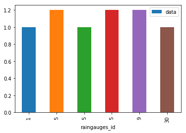
Select a subset of rows in the rainfall_df DataFrame that contain data from 4th of December and that contain rainfall values larger than or equal to 1.
How many rows did you end up with? What did your neighbor get? Can you make a plot of the data, e.g. with raingauge_ids on x and rainfall data on y?
You can use the isin command in Python to query a DataFrame based upon a list of values as follows:
rainfall_df[rainfall_df['raingauges_id'].isin([listGoesHere])]
Use the isin function to find all rainfall data from the raingauges from city engineers, pinetown and umlazi (hint: first look up the correct name for these raingauges). How many records contain these values?
Experiment with other queries. Create a query that finds all rows with a rainfall value equal to 0.

The ~ symbol in Python can be used to return the OPPOSITE of the selection that you specify in Python. It is equivalent to is not in. Write a query that selects all rows with region NOT equal to ‘Southern’ or ‘Northern’ in the rainfall data.
Did you get #1 right?
# subset data
rainfall_d4_gr1 = rainfall_df[(rainfall_df.day == 4) & (rainfall_df.data >= 1)]
# make plot
rainfall_d4_gr1.plot(x = 'raingauges_id', y = 'data', kind = 'bar')
Did you get #4 right?

It is a bit tricky where to put the ~. If our ‘isin’ query would look like:
rainfall_df[rainfall_df['region'].isin(['Southern','Northern'])]
 # and to better see the output let's make it:
rainfall_df[rainfall_df['region'].isin(['Southern','Northern'])][['ID','raingauges_id','region']].head()
yielding:
     ID  raingauges_id    region
2895  44              6  Northern
2896  45              6  Northern
2897  46              6  Northern
2898  47              6  Northern
2899  48              6  Northern
we need to place the ~ before the rainfall_df at the beginning of the query, i.e. rainfall_df[~rainfall_df['region']...
rainfall_df[~rainfall_df['region'].isin(['Southern','Northern'])][['ID','raingauges_id','region']].head()
yielding:
   ID  raingauges_id   region
0   1              1  Central
1   2              1  Central
2   3              1  Central
3   4              1  Central
4   5              1  Central

Using masks to identify a specific condition

A mask can be useful to locate where a particular subset of values exists or doesn’t exist - for example, NaN, or “Not a Number” values. To understand masks, we also need to understand BOOLEAN objects in Python.

Boolean values include True or False. For example,

# set x to 5
x = 5

# what does the code below return?
x > 5

# how about this?
x == 5

When we ask Python what the value of x > 5 is, we get False. This is because the condition,x is not greater than 5, is not met since x is equal to 5.

To create a boolean mask:

Set the True / False criteria (e.g. values > 5 = True)
Python will then assess each value in the object to determine whether the value meets the criteria (True) or not (False).
Python creates an output object that is the same shape as the original object, but with a True or False value for each index location.

Let’s try this out. Let’s identify all raingauges in the survey data that have null (missing or NaN) data values. We can use the isnull function to do this. The isnull function will compare each cell with a null value. If an element has a null value, it will be assigned a value of True in the output object.

pd.isnull(rainfall_df)

A snippet of the output is below:

         ID     UT   year  month    day   time  raingauges_id   name  ward_id  \
   False  False  False  False  False  False          False  False    False   
   False  False  False  False  False  False          False  False    False   
   False  False  False  False  False  False          False  False    False   
   False  False  False  False  False  False          False  False    False   
   False  False  False  False  False  False          False  False    False   
   False  False  False  False  False  False          False  False    False   
   False  False  False  False  False  False          False  False    False   
   False  False  False  False  False  False          False  False    False   
   False  False  False  False  False  False          False  False    False   
   False  False  False  False  False  False          False  False    False   
  False  False  False  False  False  False          False  False    False   
  False  False  False  False  False  False          False  False    False   
  False  False  False  False  False  False          False  False    False   
  False  False  False  False  False  False          False  False    False   
  False  False  False  False  False  False          False  False    False   
  False  False  False  False  False  False          False  False    False   
  False  False  False  False  False  False          False  False    False   
  False  False  False  False  False  False          False  False    False   
  False  False  False  False  False  False          False  False    False   
  False  False  False  False  False  False          False  False    False   
  False  False  False  False  False  False          False  False    False   
  False  False  False  False  False  False          False  False    False   
  False  False  False  False  False  False          False  False    False   
  False  False  False  False  False  False          False  False    False   
  False  False  False  False  False  False          False  False    False   
  False  False  False  False  False  False          False  False    False   
  False  False  False  False  False  False          False  False    False   
  False  False  False  False  False  False          False  False    False   
  False  False  False  False  False  False          False  False    False   
  False  False  False  False  False  False          False  False    False   
    ...    ...    ...    ...    ...    ...            ...    ...      ...   
False  False  False  False  False  False          False  False    False   
False  False  False  False  False  False          False  False    False   
False  False  False  False  False  False          False  False    False   
False  False  False  False  False  False          False  False    False   
False  False  False  False  False  False          False  False    False   
False  False  False  False  False  False          False  False    False   
False  False  False  False  False  False          False  False    False   
False  False  False  False  False  False          False  False    False   
False  False  False  False  False  False          False  False    False   
False  False  False  False  False  False          False  False    False   
False  False  False  False  False  False          False  False    False   
False  False  False  False  False  False          False  False    False   
False  False  False  False  False  False          False  False    False   
False  False  False  False  False  False          False  False    False   
False  False  False  False  False  False          False  False    False   
False  False  False  False  False  False          False  False    False   
False  False  False  False  False  False          False  False    False   
False  False  False  False  False  False          False  False    False   
False  False  False  False  False  False          False  False    False   
False  False  False  False  False  False          False  False    False   
False  False  False  False  False  False          False  False    False   
False  False  False  False  False  False          False  False    False   
False  False  False  False  False  False          False  False    False   
False  False  False  False  False  False          False  False    False   
False  False  False  False  False  False          False  False    False   
False   True  False  False  False  False          False  False     True   
False   True  False  False  False  False          False  False     True   
False   True  False  False  False  False          False  False     True   
False   True  False  False  False  False          False  False     True   
False   True  False  False  False  False          False  False     True   

      region   data  
    False  False  
    False  False  
    False  False  
    False  False  
    False  False  
    False  False  
    False  False  
    False  False  
    False  False  
    False  False  
   False  False  
   False  False  
   False  False  
   False  False  
   False  False  
   False  False  
   False  False  
   False  False  
   False  False  
   False  False  
   False  False  
   False  False  
   False  False  
   False  False  
   False  False  
   False  False  
   False  False  
   False  False  
   False  False  
   False  False  
     ...    ...  
 False  False  
 False  False  
 False  False  
 False  False  
 False  False  
 False  False  
 False  False  
 False  False  
 False  False  
 False  False  
 False  False  
 False  False  
 False  False  
 False  False  
 False  False  
 False  False  
 False  False  
 False  False  
 False  False  
 False  False  
 False  False  
 False  False  
 False  False  
 False  False  
 False  False  
 False   True  
 False   True  
 False   True  
 False   True  
 False   True  

[6749 rows x 11 columns]

To select the rows where there are null values, we can use the mask as an index to subset our data as follows:

# To select just the rows with NaN values, we can use the 'any()' method
rainfall_df[pd.isnull(rainfall_df).any(axis=1)]

We can run isnull on a particular column too. What does the code below do?

# what does this do?
empty_data = rainfall_df[pd.isnull(rainfall_df['data'])]['data']
print(empty_data)

Let’s take a minute to look at the statement above. We are using the Boolean object pd.isnull(rainfall_df['data']) as an index to rainfall_df. We are asking Python to select rows that have a NaN value of rainfall.

Challenge - Putting it all together

Create a new DataFrame that does not contain nan values for the ward_id and here rainfall values are greater than 0.

Missing Data Values - NaN

By now you probably wondered about the NaNs in the data, e.g. in the data column. NaN stands for Not a Number. NaN values are undefined values that cannot be represented mathematically. Pandas, for example, will read an empty cell in a CSV or Excel sheet as a NaN. NaNs have some desirable properties: if we were to average the data column without replacing our NaNs, Python would know to skip over those cells.

rainfall_df['data'].mean()
0.37230130486357743

Dealing with missing data values is always a challenge. It’s sometimes hard to know why values are missing - was it because of a data entry error? Or data that someone was unable to collect? Should the value be 0? We need to know how missing values are represented in the dataset in order to make good decisions. If we’re lucky, we have some metadata that will tell us more about how null values were handled.

For instance, in some disciplines, like Remote Sensing, missing data values are often defined as -9999. Having a bunch of -9999 values in your data could really alter numeric calculations. Often in spreadsheets, cells are left empty where no data are available. Pandas will, by default, replace those missing values with NaN. However it is good practice to get in the habit of intentionally marking cells that have no data, with a no data value! That way there are no questions in the future when you (or someone else) explores your data.

Where Are the NaN’s?

Let’s explore the NaN values in our data a bit further. Using the tools we learned in lesson 02, we can figure out how many rows contain NaN values for rainfall. We can also create a new subset from our data that only contains rows with rainfall values >= 0 (i.e. select meaningful rainfall values):

len(rainfall_df[pd.isnull(rainfall_df.data)])
# how many rows have data values?
len(rainfall_df[rainfall_df.data>= 0])

We can replace all NaN values with zeroes using the .fillna() method (after making a copy of the data so we don’t lose our work):

df1 = rainfall_df.copy()
# fill all NaN values with 0
df1['data'] = df1['data'].fillna(0)
df1.tail()

However NaN and 0 yield different analysis results. The mean value when NaN values are replaced with 0 is different from when NaN values are simply thrown out or ignored.

rainfall_df['data'].mean()
0.37230130486357743
df1['data'].mean()
0.3720254852570701

We can fill NaN values with any value that we chose. The code below fills all NaN values with a mean for all rainfall values.

 df1['data'] = rainfall_df['data'].fillna(rainfall_df['data'].mean())
df1.tail()

We could also chose to create a subset of our data, only keeping rows that do not contain NaN values. .dropna() removes all rows with NaNs.

df_na = rainfall_df.dropna()

If we check len(df_na) we find that the DataFrame has 6744 rows and 11 columns, 5 rows shorter than the 6749 rows original.

Useful options for .dropna are: .dropna(how = 'all') –> removes only rows where all columns have NaN, .dropna(subset=['data']) –> removes only rows that have NaN in data column.

The point is to make conscious decisions about how to manage missing data. This is where we think about how our data will be used and how these values will impact the scientific conclusions made from the data.

Python gives us all of the tools that we need to account for these issues. We just need to be cautious about how the decisions that we make impact scientific results.

Challenge - Counting

Count the number of missing values per column. Hint: The method .count() gives you the number of non-NA observations per column. Try looking to the .isnull() method.

Writing Out Data to CSV

We’ve learned about using manipulating data to get desired outputs. But we’ve also discussed keeping data that has been manipulated separate from our raw data. Something we might be interested in doing is working with only the columns that have full data. First, let’s reload the data so we’re not mixing up all of our previous manipulations.

rainfall_df = pd.read_csv("data/rainfall_combined.csv")

Then let’s drop all rows with NaNs.

rainfall_na = rainfall_df.dropna()

We can now use the to_csv command to export a DataFrame in CSV format. Note that the code below will by default save the data into the current working directory. We can save it to a different folder by adding the foldername and a slash to the file df.to_csv('foldername/out.csv'). We use the index=False so that pandas doesn’t include the index number for each line.

# Write DataFrame to CSV
rainfall_na.to_csv('data_output/rainfall_complete.csv', index=False)

We will use this data file later in the workshop. Check out your working directory to make sure the CSV wrote out properly, and that you can open it! If you want, try to bring it back into python to make sure it imports properly.

Key Points

use column labels in [] to access individual columns

indexing starts at 0, when choosing a range, the stop bound is one step BEYOND the row you want to select

using the = operator, like in y = x, does not create a copy of x, instead y refers to the same object as x, the .copy() method creates a true copy

use label based loc and index based iloc for subsetting rows and columns in dataframes

we can also using criteria with ==, >, <, != etc. in subsetting

missing values in form of NaN can be dropped with .dropna()

.to_csv saves a dataframe as a csv file

previous episode

Python for data analysis

next episode

Indexing, Slicing and Subsetting DataFrames in Python

Overview

Loading our data

Indexing and Slicing in Python

Selecting data using Labels (Column Headings)

Extracting Range based Subsets: Slicing

Challenge - Extracting data

Slicing Subsets of Rows in Python

Copying Objects vs Referencing Objects in Python

Slicing Subsets of Rows and Columns in Python

Challenge - Range

Subsetting Data using Criteria

Python Syntax Cheat Sheet

Challenge - Queries

Did you get #1 right?

Did you get #4 right?

Using masks to identify a specific condition

Challenge - Putting it all together

Missing Data Values - NaN

Where Are the NaN’s?

Challenge - Counting

Writing Out Data to CSV

Key Points

previous episode

next episode