Manipulating DataFrames with pandas
Overview
Teaching: 30 min
Exercises: 30 minQuestions
How can I reshape DataFrames and make tables?
Can I work with data from multiple sources?
How can I combine data from different data sets?
Objectives
Reshape data by making pivot_tables and melting tables. - Combine data from multiple files into a single DataFrame using merge and concat. - Combine two DataFrames using a unique ID found in both DataFrames. - Join DataFrames using common fields (join keys).
Reshaping DataFrames
Many analyses and statistical functions require for the data to be in a specific format. We learned about the so-called “long” and “wide” format earlier. Pandas DataFrames have methods to change between these formats.
Let’s say we want to summarise rainfall for the individual raingauges per day and want to have the rainfall spread out with one column for each day and one row for each raingauge (wide format or matrix like or ).
We can use
rainfall_day = rainfall_df.groupby(by=['day','raingauges_id']).sum()
to summarise per day and raingauge, but then we will still have all the rainfall values in one column.
Note, that the two grouping variables raingauges_id and day now appear as an index, not a column. If we want them as columns again we can use
rainfall_day = rainfall_day.reset_index()
To reshape the DataFrame after summarising it we can use method .pivot(). pivot() takes the arguments index, columns, and values.
With index we define which variable should be spreasd out into rows, i.e. 'raingauges_id' in our example; with columns we define the variable we want to turn into several columns, i.e. 'day' in our example; and with values we tell Python which variable holds the measurements we want to fill in, i.e. 'data' in our example.
rainfall_day_wide = rainfall_day.pivot(index='raingauges_id',columns='day', values='data')
rainfall_day.head()

day             1         2         3         4         5         6         7
raingauges_id
1             NaN  0.360000  0.333333  0.304348  0.257143  0.369620  0.200000
2             NaN  0.133333  0.733333  0.208696  0.397101  0.316667  0.200000
3             NaN  0.000000  0.800000  0.200000  0.323810  0.234568       NaN
4             NaN  0.733333  0.133333  0.266667  0.297674  0.370093  0.733333
5             NaN  0.200000  0.333333  0.340000  0.286207  0.472897  0.200000
Note, that raingauges_id now appears as the index, not a column, the 7 days are the columns.
If we need the raingauges_id values to be presented in a column, we can use:
# reset_index to get column with raingauges_id
rainfall_day_wide = rainfall_day_wide.reset_index()
Also note the nan values that were introduced when there was no rainfall value for a day - raingauge combination.
Getting data back into long format
We can take the rainfall_day_wide DataFrame we just created and reshape it into the “long” format, i.e. one column with raingauge_ids, one column with days and one column with the measured values using the method .melt(). melt() needs the information which columns are index- or key-variables and which colums are values, i.e. measured data (when defining id variables melt assumes by default that all other columns are values):
# melt data with raingauges_id as id variable
rainfall_day_long = rainfall_day_wide.melt(id_vars='raingauges_id', var_name='day')
Challenge
Summarise data per region and day and reshape the data so that they have one column per region and the days as row index using
group_by()andpivot().Optional: Instead of using
group_by()to summarise the data andpivot()to reshape, try to do both at once using the functionpivot_table().How to use pivot_table
rainfall_day_wide = rainfall_data.pivot_table(values='data', index='day', columns='region', aggfunc='sum')
Combining DataFrames
In many “real world” situations, the data that we want to use come in multiple
files. We often need to combine these files into a single DataFrame to analyze
the data. The pandas package provides various methods for combining
DataFrames including
merge and concat.
To work through the examples below, we first need to load the different files into pandas DataFrames. We will work with the files ‘raingauge_data.csv’, ‘raingauges.csv’ and ‘region.csv’.
(If done SQL already remember the files from there, otherwise open in text editor for first look)
import pandas as pd
rain_df = pd.read_csv("data/raingauge_data.csv")
rain_df.head()
gauges_df = pd.read_csv("data/raingauges.csv")
gauges_df.head()
  id                  name  location_x  location_y  region_id reference  \
0   1        BLUFF RES NO.3   31.005075  -29.933965          1    bluff3
1   2   CHATSWORTH RES NO.1   30.900285  -29.911171          1    chats1
2   3   CHATSWORTH RES NO.4   30.859903  -29.903620          1    chats4
3   4  CITY ENGINEER'S DEPT   31.023634  -29.851328          1   cityeng
4   5        CRABTREE S-P-S   30.992646  -29.883997          1  crabtree

   ward_id
0       66
1       70
2       71
3       26
4       32
regions_df = pd.read_csv("data/regions.csv", names=('id','region'))
regions_df.head()
Take note that the read_csv method we used can take some additional options which
we didn’t use previously. Many functions in python have a set of options that
can be set by the user if needed. In this case we used name to hand over a list with column names, since the region.csv file missed column names.
More about all of the read_csv options here.
Concatenating DataFrames
We can use the concat function in Pandas to append either columns or rows from
one DataFrame to another. Let’s grab two subsets of our data to see how this works.
# read in first 10 lines of rain table
rain_sub = rain_df.head(10)
# grab the last 10 rows
rain_sub_last10 = rain_df.tail(10)
#reset the index values to the second dataframe appends properly
survey_sub_last10=survey_sub_last10.reset_index(drop=True)
# drop=True option avoids adding new index column with old index values
When we concatenate DataFrames, we need to specify the axis. axis=0 tells
Pandas to stack the second DataFrame under the first one. It will automatically
detect whether the column names are the same and will stack accordingly.
axis=1 will stack the columns in the second DataFrame to the RIGHT of the
first DataFrame. To stack the data vertically, we need to make sure we have the
same columns and associated column format in both datasets. When we stack
horizontally, we want to make sure what we are doing makes sense (ie the data are
related in some way).
# stack the DataFrames on top of each other
vertical_stack = pd.concat([rain_sub, rain_sub_last10], axis=0)

# place the DataFrames side by side
horizontal_stack = pd.concat([rain_sub, rain_sub_last10], axis=1)
Row Index Values and Concat
Have a look at the vertical_stack dataframe? Notice anything unusual?
The row indexes for the two data frames rain_sub and rain_sub_last10
have been repeated. We can reindex the new dataframe using the reset_index() method.
vertical_stack.reset_index(drop=True)
Challenge - Combine Data
In the data folder, there are two rainfall data files:
rainfallNorth.csvandrainfallSouth.csv. Read the data into python and combine the files to make one new data frame. Export your results as a CSV and make sure it reads back into python properly.
Joining DataFrames
When we concatenated our DataFrames we simply added them to each other - stacking them either vertically or side by side. Another way to combine DataFrames is to use columns in each dataset that contain common values (a common unique id). Combining DataFrames using a common field is called “joining”. The columns containing the common values are called “join key(s)”. Joining DataFrames in this way is often useful when one DataFrame is a “lookup table” containing additional data that we want to include in the other.
NOTE: This process of joining tables is similar to what we do with tables in an SQL database.
For example, the raingauges.csv and the regions.csv file are lookup
tables. The raingauges.csv table contains the name, x and y coordinates, and a short reference for the 42 raingauges. The
raingauges id is unique for each line. These raingauges are identified in our rainfall
data as well using the unique id. Rather than adding more columns
for the name, location etc to each of the 6,749 lines in the rainfall data table, we
can maintain the shorter table with the raingauges information. When we want to
access that information, we can create a query that joins the additional columns
of information to the rainfall data.
Storing data in this way has many benefits including:
- It ensures consistency in the spelling of raingauge attributes (name, reference …) given each raingauge is only entered once. Imagine the possibilities for spelling errors when entering the raingauge names thousands of times!
- It also makes it easy for us to make changes to the raingauge information once without having to find each instance of it in the larger rainfall data.
- It optimizes the size of our data.
Joining Two DataFrames
# read in rainfall data
rain_df = pd.read_csv('data/raingauge_data.csv')

# read in raingauge infos
gauges_df = pd.read_csv('data/raingauges.csv')
In this example, gauges_df is the lookup table containing name and location of raingauges that we want to join with the data in rain_df to produce a new DataFrame that contains all of the columns from both rain_df and
gauges_df.
Identifying join keys
To identify appropriate join keys we first need to know which field(s) are shared between the files (DataFrames). We might inspect both DataFrames to identify these columns. If we are lucky, both DataFrames will have columns with the same name that also contain the same data. If we are less lucky, we need to identify a (differently-named) column in each DataFrame that contains the same information.
gauges_df.columns

Index(['id', 'name', 'location_x', 'location_y', 'region_id', 'reference', 'ward_id'],
      dtype='object')

rain_df.columns

Index(['ID', 'UT', 'data', 'raingauges_id'], dtype='object')
In our example, the join key is the column containing the id (integer between 1 and 44) for the raingauge, which is called id in the gauges table and raingauges_id in the rain table.
Now that we know the fields with the common raingauge ID attributes in each DataFrame, we are almost ready to join our data. However, since there are different types of joins, we also need to decide which type of join makes sense for our analysis.
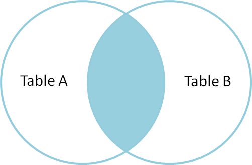
Inner joins
The most common type of join is called an inner join. An inner join combines two DataFrames based on a join key and returns a new DataFrame that contains only those rows that have matching values in both of the original DataFrames.
Inner joins yield a DataFrame that contains only rows where the value exists in BOTH tables. An example of an inner join, adapted from this page is below:
The pandas function for performing joins is called merge and an Inner join is
the default option:
merged_inner = pd.merge(left=rain_df,right=gauges_df, left_on='raingauges_id', right_on='id')
# since the keys have different names (`raingauges_id` and `id`) in the two dataframes we have to define the join keys with `left_on` and `right_on`. If the join keys would have the same name we could skip `left_on` and `right_on`

# what's the size of the output data?
merged_inner.shape
merged_inner.head()
OUTPUT:
The result of an inner join of rain_df and gauges_df is a new DataFrame
that contains the combined set of columns from rain_df and gauges_df. It
only contains rows that have raingauge ids that are the same in
both the rain_df and gauges_df DataFrames. In other words, if a row in
rain_df has a value of raingauges_id that does not appear in the id
column of gauges_df, it will not be included in the DataFrame returned by an
inner join. Similarly, if a row in gauges_df has a value of id
that does not appear in the raingauges_id column of rain_df, that row will not
be included in the DataFrame returned by an inner join.
The two DataFrames that we want to join are passed to the merge function using
the left and right argument. The left_on='raingauges_id' argument tells merge
to use the raingauges_id column as the join key from rain_sub (the left
DataFrame). Similarly , the right_on='id' argument tells merge to
use the id column as the join key from gauges_df (the right
DataFrame). For inner joins, the order of the left and right arguments does
not matter.
The result merged_inner DataFrame contains all of the columns from rain_df
(ID, UT, data etc.) as well as all the columns from gauges_df
(id, name, location_x, etc).
In our case merged_inner has fewer rows than rain_df. This is an
indication that there were rows in rain_df with value(s) for raingauges_id that
do not exist as value(s) for id in gauges_df.
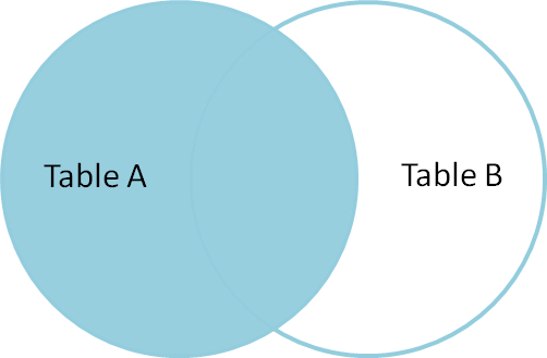
Left joins
What if we want to add information from gauges_df to rain_df without
losing any of the information from rain_df? In this case, we use a different
type of join called a “left outer join”, or a “left join”.
Like an inner join, a left join uses join keys to combine two DataFrames. Unlike
an inner join, a left join will return all of the rows from the left
DataFrame, even those rows whose join key(s) do not have values in the right
DataFrame. Rows in the left DataFrame that are missing values for the join
key(s) in the right DataFrame will simply have null (i.e., NaN or None) values
for those columns in the resulting joined DataFrame.
Note: a left join will still discard rows from the right DataFrame that do not
have values for the join key(s) in the left DataFrame.
A left join is performed in pandas by calling the same merge function used for
inner join, but using the how='left' argument:
merged_left = pd.merge(left=survey_sub,right=species_sub, how='left', left_on='species_id', right_on='species_id')

merged_left
OUTPUT:
         ID          UT  data  raingauges_id    id                  name  \
0         1  1512227100   0.6              1   1.0        BLUFF RES NO.3
1         2  1512227400   0.8              1   1.0        BLUFF RES NO.3
2         3  1512227700   0.2              1   1.0        BLUFF RES NO.3
3         4  1512228000   0.2              1   1.0        BLUFF RES NO.3
4         5  1512252000     0              1   1.0        BLUFF RES NO.3
5         6  1512325800   0.2              1   1.0        BLUFF RES NO.3
6         7  1512326100   0.2              1   1.0        BLUFF RES NO.3
7         8  1512326400   0.4              1   1.0        BLUFF RES NO.3
8         9  1512326700   0.8              1   1.0        BLUFF RES NO.3
9        10  1512327000   0.4              1   1.0        BLUFF RES NO.3
10       11  1512338400     0              1   1.0        BLUFF RES NO.3
11       12  1512226800   0.2              2   2.0   CHATSWORTH RES NO.1
12       13  1512227100   0.2              2   2.0   CHATSWORTH RES NO.1
13       14  1512252000     0              2   2.0   CHATSWORTH RES NO.1
14       15  1512325500   0.2              2   2.0   CHATSWORTH RES NO.1
15       16  1512325800   0.6              2   2.0   CHATSWORTH RES NO.1
16       17  1512326100   1.6              2   2.0   CHATSWORTH RES NO.1
17       18  1512326400   1.8              2   2.0   CHATSWORTH RES NO.1
18       19  1512326700   0.2              2   2.0   CHATSWORTH RES NO.1
19       20  1512338400     0              2   2.0   CHATSWORTH RES NO.1
20       21  1512252000     0              3   3.0   CHATSWORTH RES NO.4
21       22  1512325500   0.4              3   3.0   CHATSWORTH RES NO.4
22       23  1512325800   1.4              3   3.0   CHATSWORTH RES NO.4
23       24  1512326100   2.6              3   3.0   CHATSWORTH RES NO.4
24       25  1512326400   0.2              3   3.0   CHATSWORTH RES NO.4
25       26  1512331800   0.2              3   3.0   CHATSWORTH RES NO.4
26       27  1512338400     0              3   3.0   CHATSWORTH RES NO.4
27       28  1512227100   1.8              4   4.0  CITY ENGINEER'S DEPT
28       29  1512227400   0.4              4   4.0  CITY ENGINEER'S DEPT
29       30  1512252000     0              4   4.0  CITY ENGINEER'S DEPT
    ...         ...   ...            ...   ...                   ...
6719  71602  1512624300   0.4             34  34.0          ISIPINGO RES
6720  71603  1512625200   0.2             34  34.0          ISIPINGO RES
6721  71604  1512626400   0.2             34  34.0          ISIPINGO RES
6722  71621  1512624300   0.2             42  42.0           AMANZIMTOTI
6723  71625  1512629100   0.2              2   2.0   CHATSWORTH RES NO.1
6724  71628  1512629100   0.2              5   5.0        CRABTREE S-P-S
6725  71647  1512627000   0.2             18  18.0         WENTWORTH RES
6726  71662  1512629100   0.2             36  36.0              RIVERLEA
6727  71678  1512633900   0.2              1   1.0        BLUFF RES NO.3
6728  71679  1512634200   0.2              1   1.0        BLUFF RES NO.3
6729  71682  1512632400   0.2              4   4.0  CITY ENGINEER'S DEPT
6730  71685  1512634200   0.2              5   5.0        CRABTREE S-P-S
6731  71686  1512634500   0.2              5   5.0        CRABTREE S-P-S
6732  71687  1512635400   0.2              5   5.0        CRABTREE S-P-S
6733  71693  1512633900   0.2              9   9.0     ISLAND VIEW S-P-S
6734  71699  1512633300   0.2             15  15.0      SAND PUMP HOPPER
6735  71716  1512633300   0.2             29  29.0         SHONGWENI DAM
6736  71717  1512632100   0.2             30  30.0              PINETOWN
6737  71734  1512633600   0.2             38  38.0               UMH NTH
6738  71774  1512634500   0.2             18  18.0         WENTWORTH RES
6739  71785  1512627600   0.4             33  33.0         UMBUMBULU RES
6740  71786  1512627900   0.4             33  33.0         UMBUMBULU RES
6741  71787  1512636300   0.2             34  34.0          ISIPINGO RES
6742  71788  1512636600   0.2             34  34.0          ISIPINGO RES
6743  71796  1512634800   0.2             35  35.0              UMKDEPOT
6744  80001  1512605100   nan             43   NaN                   NaN
6745  80002  1512606000   nan             43   NaN                   NaN
6746  80003  1512606600   nan             43   NaN                   NaN
6747  80004  1512606900   nan             43   NaN                   NaN
6748  80005  1512608700   nan             43   NaN                   NaN

      location_x  location_y  region_id reference  ward_id
0      31.005075  -29.933965        1.0    bluff3     66.0
1      31.005075  -29.933965        1.0    bluff3     66.0
2      31.005075  -29.933965        1.0    bluff3     66.0
3      31.005075  -29.933965        1.0    bluff3     66.0
4      31.005075  -29.933965        1.0    bluff3     66.0
5      31.005075  -29.933965        1.0    bluff3     66.0
6      31.005075  -29.933965        1.0    bluff3     66.0
7      31.005075  -29.933965        1.0    bluff3     66.0
8      31.005075  -29.933965        1.0    bluff3     66.0
9      31.005075  -29.933965        1.0    bluff3     66.0
10     31.005075  -29.933965        1.0    bluff3     66.0
11     30.900285  -29.911171        1.0    chats1     70.0
12     30.900285  -29.911171        1.0    chats1     70.0
13     30.900285  -29.911171        1.0    chats1     70.0
14     30.900285  -29.911171        1.0    chats1     70.0
15     30.900285  -29.911171        1.0    chats1     70.0
16     30.900285  -29.911171        1.0    chats1     70.0
17     30.900285  -29.911171        1.0    chats1     70.0
18     30.900285  -29.911171        1.0    chats1     70.0
19     30.900285  -29.911171        1.0    chats1     70.0
20     30.859903  -29.903620        1.0    chats4     71.0
21     30.859903  -29.903620        1.0    chats4     71.0
22     30.859903  -29.903620        1.0    chats4     71.0
23     30.859903  -29.903620        1.0    chats4     71.0
24     30.859903  -29.903620        1.0    chats4     71.0
25     30.859903  -29.903620        1.0    chats4     71.0
26     30.859903  -29.903620        1.0    chats4     71.0
27     31.023634  -29.851328        1.0   cityeng     26.0
28     31.023634  -29.851328        1.0   cityeng     26.0
29     31.023634  -29.851328        1.0   cityeng     26.0
         ...         ...        ...       ...      ...
6719   30.923468  -30.014299        4.0  isipingo     93.0
6720   30.923468  -30.014299        4.0  isipingo     93.0
6721   30.923468  -30.014299        4.0  isipingo     93.0
6722   30.866731  -30.048904        4.0   amanzim     97.0
6723   30.900285  -29.911171        1.0    chats1     70.0
6724   30.992646  -29.883997        1.0  crabtree     32.0
6725   30.988069  -29.934086        1.0   wentwth     68.0
6726   30.294999  -29.880668        3.0  riverlea      3.0
6727   31.005075  -29.933965        1.0    bluff3     66.0
6728   31.005075  -29.933965        1.0    bluff3     66.0
6729   31.023634  -29.851328        1.0   cityeng     26.0
6730   30.992646  -29.883997        1.0  crabtree     32.0
6731   30.992646  -29.883997        1.0  crabtree     32.0
6732   30.992646  -29.883997        1.0  crabtree     32.0
6733   31.033217  -29.895545        1.0  islandvw     66.0
6734   31.050144  -29.872875        1.0  sandpump     26.0
6735   30.722337  -29.860570        3.0  shongdam      7.0
6736   30.861785  -29.816873        3.0       ptn     18.0
6737   31.077676  -29.730088        2.0    umhnth     35.0
6738   30.988069  -29.934086        1.0   wentwth     68.0
6739   30.707848  -29.981689        4.0  umbumbul      3.0
6740   30.707848  -29.981689        4.0  umbumbul      3.0
6741   30.923468  -30.014299        4.0  isipingo     93.0
6742   30.923468  -30.014299        4.0  isipingo     93.0
6743   30.754047  -30.200036        4.0  umkdepot     99.0
6744         NaN         NaN        NaN       NaN      NaN
6745         NaN         NaN        NaN       NaN      NaN
6746         NaN         NaN        NaN       NaN      NaN
6747         NaN         NaN        NaN       NaN      NaN
6748         NaN         NaN        NaN       NaN      NaN

[6749 rows x 11 columns]
The result DataFrame from a left join (merged_left) looks very much like the
result DataFrame from an inner join (merged_inner) in terms of the columns it
contains. However, unlike merged_inner, merged_left contains the same
number of rows as the original rain_df DataFrame. When we inspect
merged_left, we find there are rows where the information that should have
come from gauges_df (i.e., name, location_x, etc) is
missing (they contain NaN values):
merged_left[ pd.isnull(merged_left.name) ]
OUTPUT:
         ID          UT  data  raingauges_id  id name  location_x  location_y  \
6744  80001  1512605100   nan             43 NaN  NaN         NaN         NaN
6745  80002  1512606000   nan             43 NaN  NaN         NaN         NaN
6746  80003  1512606600   nan             43 NaN  NaN         NaN         NaN
6747  80004  1512606900   nan             43 NaN  NaN         NaN         NaN
6748  80005  1512608700   nan             43 NaN  NaN         NaN         NaN

      region_id reference  ward_id
6744        NaN       NaN      NaN
6745        NaN       NaN      NaN
6746        NaN       NaN      NaN
6747        NaN       NaN      NaN
6748        NaN       NaN      NaN
These rows are the ones where the value of raingauges_id from rain_df (in this
case, 43) does not occur in gauges_df.
Other join types
The pandas merge function supports two other join types:
- Right (outer) join: Invoked by passing
how='right'as an argument. Similar to a left join, except all rows from therightDataFrame are kept, while rows from theleftDataFrame without matching join key(s) values are discarded. - Full (outer) join: Invoked by passing
how='outer'as an argument. This join type returns the all pairwise combinations of rows from both DataFrames; i.e., the result DataFrame willNaNwhere data is missing in one of the dataframes. This join type is very rarely used.
Final Challenges
Challenge
Create a new DataFrame by joining the contents of the
raingauge_data.csvandraingauges.csvtables. Then summarise the data (rainfall) over:
- raingauges by region_id
- raingauges by day by region_id
In the data folder, there is a region
CSVthat contains information about the region associated with each raingauge. Use that data together with theraingaugestable to count the raingauges per region and show the raingauges names per region name.
Key Points
the method .pivot_table() creates pivot tables or can just be used to reshape data from long to wide format
the method .melt() brings data back to long format
the function pd.concat() can be used to concatenate/stack two DataFrames
axis = 0 will stack vertically and axis = 1 horizontally
the function pd.merge() can be used to join two DataFrames and requires joining keys
pandas can perform inner joins, the default option in merge(), left joins, right joins and full joins